compiling distributed ML systems

20 Sep 2024

Alpa

Alpa is a library that automates model-parallel training for larg deep learning models: it automatically generates execution plans that unify data, operator, and pipeline parallelism. Its key idea is viewing parallelisms in two hierarchical levels: inter-operator and intra-operator. It designs compilation passes to automatically derive efficient parallel execution plans at each parallelism level.

Basics and Definitions

The conventional view of ML parallelization approaches splits them into three categories:

Data parallelism: partitions the data across devices and trains the model on each partition in parallel. After each worker computes parameter updates on its data split, it needs to synchronize with other workers before performing a weight update.
Operator parallelism: partitions the computatin of an operator (e.g. a matmul) along non-batch axes and compute each part of that operator in parallel across multiple devices. This strategy requires communication to fetch input data from other devices.
Pipeline parallelism: places different groups of ops from the model graph (stages) on different workers, splits the training batch into microbatches, and pipelines the forward and backward passes across microbatches on distributed workers.

While approaches such as Megatron-LM manually combine theses three parallelisms, explorations of auto-parallelization relying on this view have limitations. Using an example from the paper: if you’re already employing operator parallelism and want to introduce data parallel replicas, you have to introduce a new set of devices and figure out the optimal operator parallelism scheme within those devices.

The key difference between the types of parallelism presented is their granularity and whether they take operators to be a basic unit.

data, operator, pipeline parallelism
intra-operator parallelism: partitions ML operators along one or more tensor axes and dispatches those partitions to distributed devies. This achieves better device utilization, but has larger communication overhead (since it needs to communicate at every split/merge of partitioned operators).
inter-operator parallelism: slices the model into disjoint stages and pipelines the execution of stages on different sets of devices. With proper slicing the communication overhead can be light, but scheduling constraints cause device idle time (see work like GPipe).

Alpa’s Strategy

Naturally, then, if you’re thinking about mapping parallelism to devices in a compute cluster, it makes sense to map intra-operator parallelism to devices with high communication bandwidth, and inter-operator parallelism to devices with less communication bandwidth. As noted, it works at two key levels:

Intra-op optimization: Minimize the cost of executing a stage of the computational graph w/r/t/ its intra-operator parallelism plan on a given device mesh (a set of devices with high inter-device bandwidth, e.g. GPUs within a server).
Inter-op optimization: Minimize inter-op parallelization latency, w/r/t/ slicing the model and device cluster into stages and device meshes and mapping into stage-mesh pairs. This requires knowing the execution cost of each stage-mesh pair reported by the intra-op optimizer.

It introduces three compiler passes, as shown below:

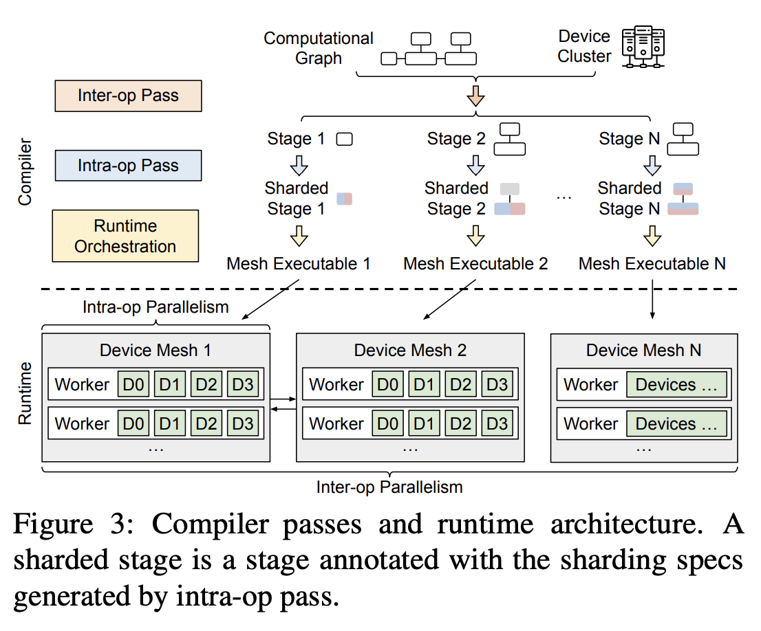
Alpa compiler passes and runtime architecture.

Given Jax IR and a cluster config, the inter-op pass slices the IR into stages, cuts the cluster into device meshes, then assigns stages to device meshes and invokes the intra-op pass on each stage-mesh pair to determine the execution cost of its assignment. It repeatedly queries the intra-op pass and uses DP to minimize inter-op parallel execution latency and achieve the best slicing scheme.

A very simplistic version (not as described in the paper) could look like this, assuming we have certain methods/types:

def inter_op_pass(jax_ir: JaxIR, cluster_config: ClusterConfig) -> List[StageMeshPair]:
    num_operators = len(jax_ir.operators)
    num_devices = cluster_config.num_devices
    
    dp = [[float('inf')] * (num_devices + 1) for _ in range(num_operators + 1)]
    dp[0][0] = 0
    backtrack = [[[]] * (num_devices + 1) for _ in range(num_operators + 1)]
    
    # DP
    for i in range(1, num_operators + 1):
        for j in range(1, num_devices + 1):
            for k in range(i):
                stage = jax_ir.operators[k:i]
                for mesh_shape in get_possible_mesh_shapes(j - k):
                    mesh = DeviceMesh.create(mesh_shape)
                    cost = intra_op_pass(stage, mesh, cluster_config)
                    if dp[k][j-len(stage)] + cost < dp[i][j]:
                        dp[i][j] = dp[k][j-len(stage)] + cost
                        backtrack[i][j] = backtrack[k][j-len(stage)] + [StageMeshPair(stage, mesh, cost)]
    
    # return best slicing scheme
    return backtrack[num_operators][num_devices]

Intra-op optimization

The intra-op pass solves an ILP to minimize its execution cost. It uses SPMD-style intra-op parallelism to reduce its search space, since SPMD partitions operators evenly across devices and executes the smae instructions on all devices. There are a few key ideas we need to understand how the intra-op pass works:

Device mesh: a 2-D logical view of a set of physical devices, where each device in a mesh has the same compute capability.
Sharding Spec: The sharding spec defines the layout of a tensor — each dimension is sharded or replicated across devices. The layout of an $N$-dimensional tensor is described as $X_0X_1…X_{N-1}$, where $X_i \in {S,R}$ indicates partitioning or replication for the $i$th dimension. For a 2-dimensional tensor, a spec $SR$ means it is row-partitioned. The authors also introduce a superscript to $S$ to denote device assignment: $S^0$ indicates partitioning along the 0th axis of a mesh, while $S^{01}$ indicates partitioning along both mesh axes.
Resharding: If the input tensor of an operator doesn’t satisfy the sharding spec of the parallel algorithm chosen for that operator, a layout conversion (resharding) is necessary.
Parallel algorithms of an operator: Based on an analysis of an operator’s expression (e.g. a batched matmul), we can work out possible algorithms — these involve a parallel mapping, an output (sharding) spec, input specs, and communication cost (e.g. all-reduce communication).

The ILP formulation for this pass uses an objective function that minimizes the sum of compute and communication costs. Its decision variables represent the choice of parallel algorithm for each op and the constraints ensure exactly one algorithm is chosen for each operator.

to work out communication costs, the authors compute the numbers of communicated bytes and divide by the mesh dimension bandwidth.
compute costs are set to zero — the authors argue that this is reasonable, since (1) we don’t allow replicated computation for heavy ops like matmul, and (2) computation costs are negligible for the lightweight operators where we do allow replication.

Here’s a heavily simplified version, assuming we have methods like get_parallel_algorithms and estimate_resharding_cost:

def intra_op_pass(operators: List[Operator], mesh: DeviceMesh) -> Dict[Operator, ParallelAlgorithm]:
    prob = pulp.LpProblem("Intra_Op_Optimization", pulp.LpMinimize)
    
    vars = {}
    for op in operators:
        for alg in get_parallel_algorithms(op, mesh):
            vars[(op, alg)] = pulp.LpVariable(f"{op.name}_{alg.input_spec}_{alg.output_spec}", cat='Binary')
    
    # objective
    prob += pulp.lpSum(vars[(op, alg)] * (alg.communication_cost + alg.computation_cost)
                       for op in operators
                       for alg in get_parallel_algorithms(op, mesh))
    
    # add constraints
    for op in operators:
        prob += pulp.lpSum(vars[(op, alg)] for alg in get_parallel_algorithms(op, mesh)) == 1
    
    # resharding costs
    for i in range(len(operators) - 1):
        op1, op2 = operators[i], operators[i+1]
        for alg1 in get_parallel_algorithms(op1, mesh):
            for alg2 in get_parallel_algorithms(op2, mesh):
                resharding_cost = estimate_resharding_cost(alg1.output_spec, alg2.input_spec, np.prod(op1.output_shape), mesh)
                prob += pulp.lpSum(vars[(op1, alg1)] * vars[(op2, alg2)] * resharding_cost)
    
    prob.solve()
    
    solution = {}
    for op in operators:
        for alg in get_parallel_algorithms(op, mesh):
            if pulp.value(vars[(op, alg)]) == 1:
                solution[op] = alg
                break
    
    return solution

Inter-op optimization

Let’s formalize inter-operator parallelism a bit more. We’ll think of the computational graph as a sequence of ops following the graph’s topological order, written as $o_1,…,o_{k-1}$. As described earlier, the operators are described into $S$ stages $s_1,\ldots,s_S$ where each stage contains operators $(o_{l_i},\ldots,o_{r_i})$ and each stage $s_i$ is assigned to a submesh of size $n_i \times m_i$, from a cluster mesh with shape $N \times M$.

The latency of executing stage $s_i$ on submesh of size $n_i \times m_i$ is written $t_i = t_{intra}(s_i,Mesh(n_i,m_i))$ — given $B$ input microbatches for the pipeline, the total minimum latency for the computation graph is given by

\begin{equation} T^* = \min_{s_1,\ldots,s_S; (n_1,m_1),\ldots,(n_S,m_S)} \left{\sum_{i=1}^S t_i + (B-1) \cdot \max_{1\leq j\leq S} {t_j}\right}. \tag{2} \end{equation}

where the first term is the total latency of all stages, and the second is the pipelined execution time for the other $B-1$ microbatches, bounded by the lowest stage. The figure below illustrates the pipeline latency:

Pipeline latency for inter-op parallelism.

The authors propose a DP algorithm to find $T^*$. [tk explain this better]

Here’s how you might write the inter-op pass, more or less based on the psudocode in Algorithm 1.

def inter_op_pass(G: ModelGraph, C: Tuple[int, int], B: int) -> float:
    N, M = C
    operators = flatten(G) # topological sort, yields (o1,...,ok)
    layers = operator_clustering(operators)
    L = len(layers)

    submesh_shapes = [(1, 2**i) for i in range(int(np.log2(M))+1)] + [(i, M) for i in range(2, N+1)] # {(1,1), (1,2), (1,4), ..., (1,M)} U {(2,M), (3,M), ..., (N,M)}
    
    t_intra = {}
    
    # t_intra for all possible stage-mesh pairs
    # recall that t_intra(s_i, Mesh(n_i, m_i)) is the minimum execution time of stage s_i on a mesh of size n_i x m_i
    for i in range(L):
        for j in range(i, L):
            stage = layers[i:j+1]
            for n, m in submesh_shapes:
                for s in range(1, L+1):
                    t_intra[(i, j, n, m, s)] = float('inf')
                for (n_l, m_l), opt in logical_mesh_shape_and_intra_op_options(n, m):
                    plan = intra_op_pass(stage, DeviceMesh((n_l, m_l)), opt)
                    t_l, mem_stage, mem_act = profile(plan)
                    for s in range(1, L+1):
                        # check whether the required memory fits the device memory
                        # in the 1 fwd 1 bwd schedule, max_stored_activations = s and this reduces to Equation 5
                        if mem_stage + max_stored_activations * mem_act <= mem_device:
                            if t_l < t_intra[(i, j, n, m, s)]:
                                t_intra[(i, j, n, m, s)] = t_l

    T_star = float('inf')
    for t_max in sorted(set(t_intra.values())):
        if B * t_max >= T_star:
            break
        
        F = {}
        F[(0, L+1, 0)] = 0
        
        for s in range(1, L+1):
            for l in range(L, 0, -1):
                for d in range(1, N*M+1):
                    F[(s, l, d)] = float('inf')
                    for k in range(l-1, -1, -1):
                        for n, m in submesh_shapes:
                            if n * m <= d and t_intra[(k, l-1, n, m, s)] <= t_max:
                                F[(s, l, d)] = min(F[(s, l, d)], 
                                                   F[(s-1, k, d-n*m)] + t_intra[(k, l-1, n, m, s)])

        T_star_t_max = min(F[(s, 0, N*M)] for s in range(1, L+1)) + (B - 1) * t_max
        if T_star_t_max < T_star:
            T_star = T_star_t_max

    return T_star

Ideas

The paper notes five different limitations.

It doesn’t handle cross-stage communication cost since that communication cost is small. This is typically true for sequential architectures, but not necessarily for models w/ skip connections or dense connectivity patterns.
Doesn’t optimize for # of microbatches B. We could adapt the DP formulation to handle this, adding DP as another dim to the optimization. This bumps the complexity of DP to $O(L^3 NMB_max)$ vs. $O(L^3NM)$.
Doesn’t consider more dynamic schedules for pipeline parallelism. I think you could also introduce schedules (e.g. GPipe) into the DP formulation — but more complexity!
Doesn’t optimize for overlapping computation and communication. Not sure how exactly this would fit into Alpa, but fine-grained scheduling is always an option: create an op dependency graph, assign each op to resources, create a time-based schedule, then schedule communication ops to overlap w/ computations that don’t depend on the communication outputs.
Only handles static computational graphs. Something with JIT compilation — idk exactly what this would look like!

Daniel Bashir