Simplifying Dependent Reductions in the Polyhedral Model

I read this really neat paper recently called “Simplifying Dependent Reductions in the Polyhedral Model” by Cambridge Yang, Eric Atkinson, and Michael Carbin. I’ll give a rundown of the main ideas: what (dependent) reductions are, why they matter (especially in ML), how this paper uses the polyhedral model to simplify them, and why that matters.

(Dependent) Reductions and why they matter:

A reduction is a pretty familiar concept: reductions combine a set of values into a single result. A reduce-add takes a list of numbers and returns their sum. A reduce-multiply takes a list of numbers and returns their product. This shows up everywhere in numerical computing, and often in ML.

Optimizing these reductions, then, can dramatically speed up workloads.

Ordinary reductions, like summing an array or finding its maximum value, have some appealing properties that make them relatively easy to optimize and parallelize: these include associativity, commutativity, and independence. Compilers and runtime systems can exploit these properties to perform parallelization, vectorization, loop unrolling, and tree-based reductions.

Dependent reductions are a different beast entirely: each step of a dependent reduction depends on the result of the previous step. This shows up in many places in numerical computing and ML, especially in convolutions, matrix multiplications, and some recurrent neural networks. The paper we’ll discuss here uses a an example of the prefix sum, but I’ll mention some examples more relevant to ML in this intro:

SGD with Momentum

The momentum update can be expressed as:

Where:

• $v_t$ is the velocity at time $t$
• $\beta$ is the momentum coefficient
• $g_t$ is the gradient at time $t$
• $\theta_t$ is the parameter at time $t$
• $\alpha$ is the learning rate

This can be expressed as a dependent reduction:

v = 0
θ = initial_params

for t in range(num_iterations):
    g_t = compute_gradient(θ)
    v = beta * v + (1 - beta) * g_t  # Dependent reduction
    θ = θ - alpha * v  # Dependent reduction

where each update to $v$ and $\theta$ depends on its previous value, forming a chain of dependent reductions.

Optimizing a reduction like this could produce significant performance improvements in training models.

Self-Attention

Attention mechanisms aren’t really implemented as dependent reductions, but certain variants (e.g. inremental self-attention in autoregressive decoding) look conceptually similar to dependent reductions.

When we compute attention scores incrementally, as below, we can express them as dependent reductions:

def incremental_self_attention(queries, keys, values, t):
    attention_scores = np.zeros((t+1, t+1))
    context_vector = np.zeros(d_model)
    
    for i in range(t+1):
        for j in range(i+1):
            attention_scores[i, j] = dot_product(queries[i], keys[j])
        
        attention_weights = softmax(attention_scores[i, :i+1])
        
        for j in range(i+1):
            context_vector += attention_weights[j] * values[j]  # Dependent reduction
    
    return context_vector

Here, the context_vector is computed incrementally, with each step depending on the previous steps.

The Polyhedral Model

The polyhedral model is a powerful technique in compiler optimization — its insight is that since programs spend most of their time in loops, it’s useful to develop a simple way to express information about loops that allows us to reason about program behavior and perform optimizations. The representation offered int he polyhedral model lets compilers analyze loopnests and dependencies, automatically find opportunities for optimization, and apply transformations to improve performance (e.g. parallelization or improving memory access patterns).

I hope to write a fuller intro in another post, but for the purposes of explaining this paper I’ll give a brief intro to how this works and show how it can be used for optimizations like reordering loops. You can understand the main heuristic algorithm in this paper without too much detail on the polyhedral model, but it’s helpful to understand it as motivation.

Some Intuition

I’ll describe the model in a bit more technical detail below, but the following might help build some intuition: the polyhedral model allows us to think about loopnests as polyhedra (hence the name) defined by the bounds of the loops that make up the loopnests (technically in more than three dimensions these are called polytopeds and the polyhedral model is also referred to as the polytope method).

If we consider a doubly-nested loop:

for (i = 0; i < N; i++) {
  for (j = 0; j <= i; j++) {
    // do something
  }
}

we can think of each iteration of the loop as a point $(i,j)$ in 2D space. The bounds of the loops define a shape containing all these points — a polygon in 2D, a polyhedron in 3D, and polytopes in higher dimensions. The loop bounds define a set of points that are valid iterations of the loop, which in this case looks like a triangle:

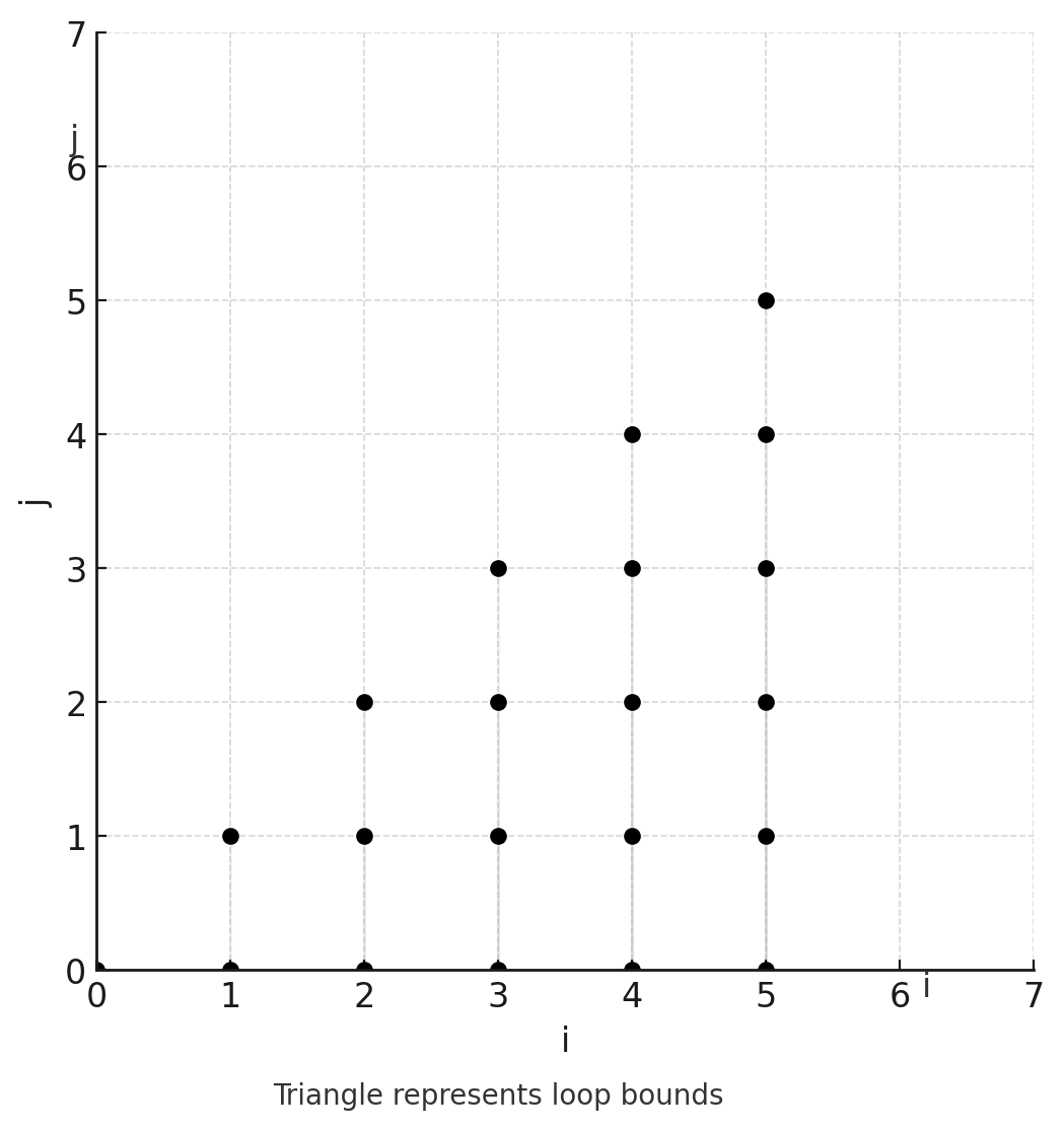
Simple loop bounds example

With a figure like this, dependencies can be represented as arrows between points. I’ll use a similar example again below with some more detail and introduce a formalization of the polyhedral model.

Representing Loops

A loop can be represented as a set of constraints on the possible values of the loop variables. For example, the loop:

for (i = 0; i < N; i++) {
    for (j = 0; j <= i; j++) {
        A[i] += B[j];
    }
}

can be represented as the constraints:

Loop iteration space example

Each point in this polyhedron represents one execution of the innermost statement (A[i] += B[j]). The coordinates of the point correspond to the values of i and j for that execution.

Formally, we define a polyhedral set as:

\(P = [p] \rightarrow \{[x] : M \cdot [x, p, 1]^T \geq 0\}\)

Where:

• $[p]$ is a vector of parameters (like $N$ in our example)
• $[x]$ is a vector of variables (like $i$ and $j$)
• $M$ is a matrix defining the inequalities

In our example:

To return to the simple example we’ve been using, we can describe the triangle with inequalities:

• $0 \leq i < N$
• $0 \leq j \leq i$

and in the polyhedral model, we can represent this as:

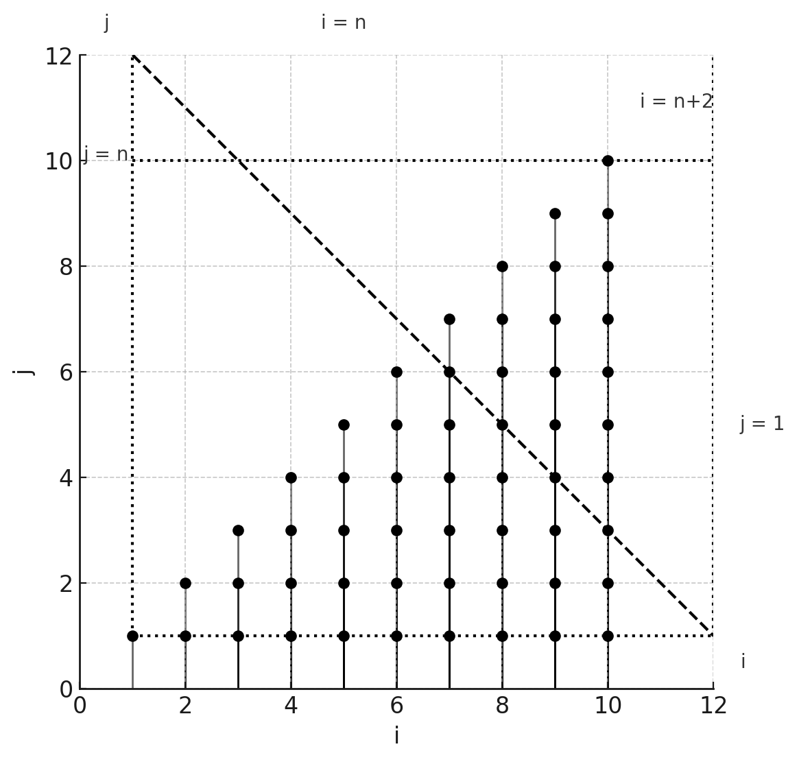
This polyhedral set defines all valid points $(i,j)$ for our loop — this is also called the iteration space of the loop. In our loop, each A[i] += B[j] operation depends on the previous iterations with the same $i$. We can represent this as arrows in our diagram.

Polyhedral reduction example with dependencies

To compute A[2], for instance, we need to perform all the additions for i=2 in order from j=0 to j=2.

In the polyhedral model we also care about schedules, which assign an execution time to each point in the iteration space. Our original loop implements the simple schedule:

meaning to execute in the order of $i$, then $j$.

This schedule can be represented more formally as a scheduling matrix. A scheduling matrix $\Theta_S$ for a statement S maps each point in the iteration space to a vector of time coordinates. For our schedule above, the scheduling matrix would look like this:

This matrix, when applied to a point $(i, j, 1)$ (we add 1 as a constant term), gives us the execution time:

Each row of the scheduling matrix corresponds to one dimension of our execution time.

If we had a different schedule:

This would swap our loop order, executing in order of $j$, then $i$. Here, the first row $\Theta_{S,1} = [0, 1, 0]$ determines the first time coordinate ($j$), and the second row $\Theta_{S,2} = [1, 0, 0]$ determines the second time coordinate ($i$).

One observation we might make is that if we reordered the original loop’s points (where we executed in the order of $i$, then $j$) in a way that still respects the dependencies, we might get a faster program (perhaps by improving memory locality, for instance).

In this case, we might realize that all the B[j] values could be summed up once, instead of repeating the sum for each i. So we write the optimized version:

sum = 0;
for (j = 0; j < N; j++) {
    sum += B[j];
    A[j] = sum;
}

In the polyhedral model, this optimization is achieved by finding a new schedule that reorders the computation while respecting dependencies.

From Independent to Dependent Reduction

As an example of a dependent reduction, the paper introduces the prefix sum — it’s exactly the loopnest we saw before:

for(i = 0; i < N; i++)
    for(j = 0; j<=i; j++)
        B[i] += A[j]

representing the summation

We would ordinarily optimize this with something called the Simplification Transformation (ST), which codifies profitably reusable computations into a set of reuse vectors. Intuitively, these vectors point from one iteration to another iteration that performs some of the same computation. Knowing about the shared computation between different loop iterations, we can restructure code to perform that shared computation once and reuse the results instead of recomputing.

In (1), the reuse vector $[1,0]^{T}$ denotes the shared computation changing $i$ to $i+1$ and $j$ to $j+0$. ST, given an equational statement like (1) and a reuse vector, transforms the statement into a set of statements that are semantically equivalent to the original statement, but reuse shared computation. Given (1) and $[1,0]^{T}$, ST would transform (1) into the following set of statements:

which has complexity $O(N)$, better than the naive $O(N^2)$ complexity of the original loop, which it achieves by setting a base case and reusing computation (like a simple DP).

We could have instead used the reuse vector $[-1,0]^{T}$ to denote the shared computation changing $i$ to $i-1$ and $j$ to $j-0$, resulting in the following set of statements:

which also has complexity $O(N)$.

To contrast with the prefix sum, which can be optimized rather easily since the input array A is not modified during the computation of B, the paper considers the following dependent reduction:

Now the reduction in (4a) is dependent because the value of the reduction $B[i]$ depends on the set of values ${A[j] \mid j \leq i}$ while $A[i]$ depends on the previous value of the reduction, $B[i-1]$. While ST works for simpler examples, applying it to dependent reductions introduces new dependencies — together with the program’s existing dependencies, the resulting program might end up with a dependence cycle.

For instance, if we had applied the reuse vector $[-1,0]^{T}$ to (4), we would have obtained a program with statements (3a), (3b), and (4b). This forms the dependence cycle $B[N-1] \rightarrow A[N-1] \rightarrow B[N-2] \rightarrow B[N-1]$. The reuse vector $[1,0]^{T}$ would have produced a valid program consisting of equations (2a), (2b), and (4b).

To illustrate valid and invalid reuse directions, let’s look at Figure 1 from the paper, which shows the iteration space of the prefix sum loop:

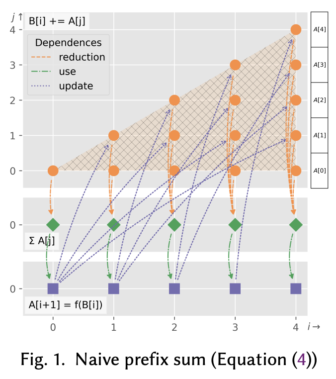
Iteration space of the prefix sum loop

The polyhedron with round dots at the top represents the iteration domain of the reduction statement B[i] += A[j] (each round dot denotes an iteration instance of the statement). The elements A[0] through A[4] on the right are the array elements A[j] to be accumulated into B[i]. The bottom polyhedron with squares it eh iteration domain for the statement A[i+1] = f(B[i]), while the middle polyhedron with diamonds is an additional polyhedron that the author’s technique inserts into a program’s polyhedral representation to denote the completion of each reduction B[i].

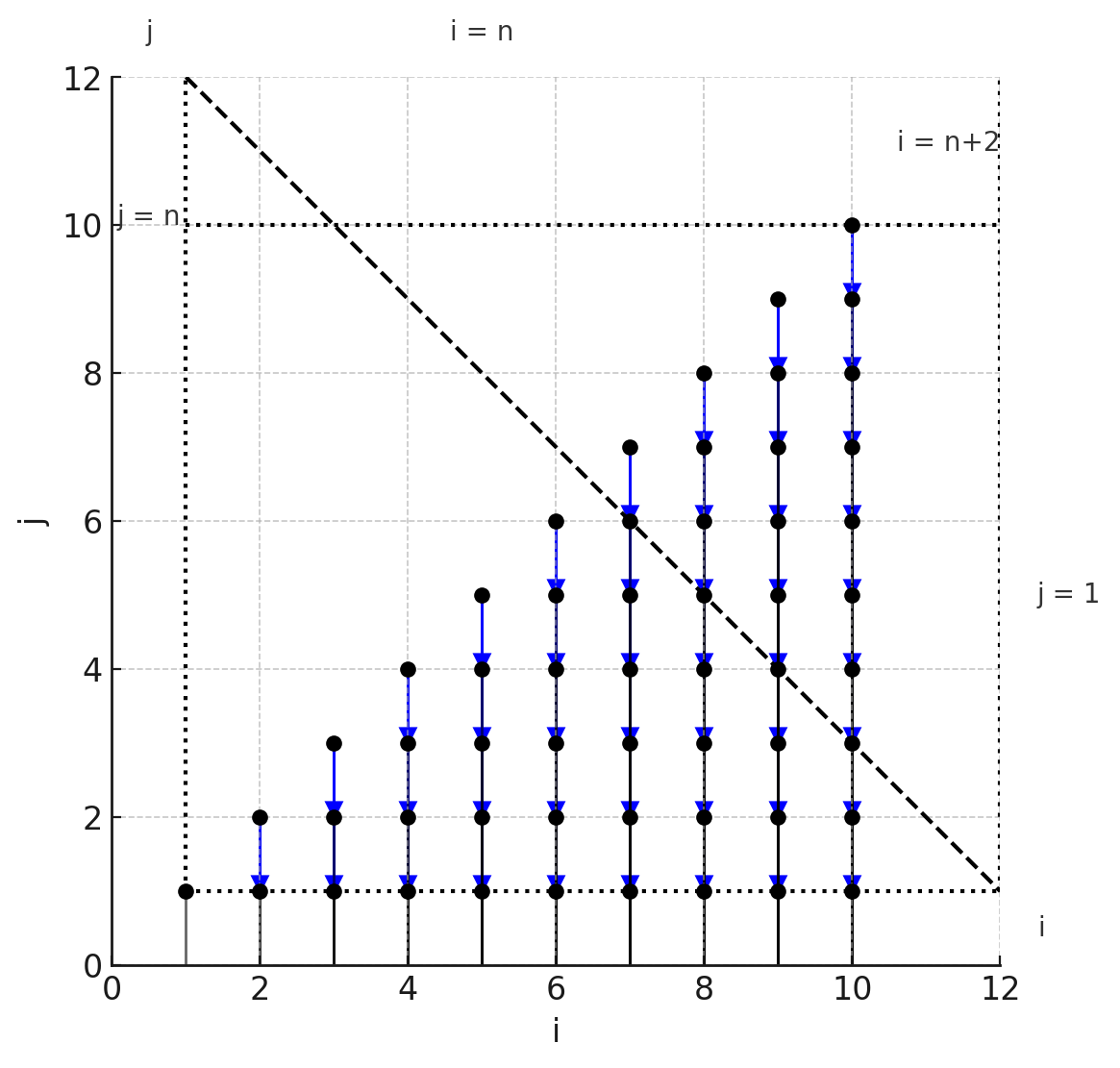
Each arrow represents a data dependency in iteration space — an arrow from $a$ to $b$ means that $a$ needs to execute before $b$. Figures 2 and 3, below, show the correct and incorrect optimizations of our dependent prefix sum with the reuse vectors $[1,0]^{T}$ and $[-1,0]^{T}$, respectively.

Correct optimization of the dependent prefix sum with the reuse vector $[1,0]^{T}$

Incorrect optimization of the dependent prefix sum with the reuse vector $[-1,0]^{T}$

An Integer Bilinear Program and a Heuristic

So, we’ve seen how the polyhedral model represents loops and how the Simplifiation Transformation (ST) can correctly and incorreclty optimize reductions. Extending techniques like ST to dependent reductions introduces the problem we saw above: how do we choose reuse vectors to simplify programs so that without introducing dependency cycles?

In the paper, the authors formulate their optimization as an Integer Bilinear Program, considering all constraints and looking for the best solution. To understand how they formulate the optimization problem, consider again the structure of polyhedral representations.

Remember our triangular iteration space for the prefix sum — that entire triangle is what we call the “domain” of our reduction. We can consider its components:

1. The entire triangle (2D face), our full iteration space.
2. The three edges of the triangle (1D faces), where one loop variable reaches its minimum or maximum value.
3. The three corners of the triangle (0D faces), where both loop variables reach their minimum/maximum values.

Each of these is called a face of the polyhedron. In the polyhedral model, a face is created when we turn some of our inequalities into equalities. For example, the bottom edge of our triangle is the face where j = 0. The paper defines a face of a polyhedral set as that polyhedral set with a subset of (potentially empty or all) inequalities changed to equality constraints.

The key insight uses this notion: instead of trying to optimize the entire reduction at once, we can think about optimizing each face separately. For each face, we want to find a “reuse vector” - a way to reuse computation from one point to another within that face.

Revisiting the prefix sum example and its iteration space:

Loop iteration space example

we can consider faces and their corresponding reuse vectors:

1. The entire triangle: Here we applied the reuse vectors $[1,0]^{T}$ and $[-1,0]^{T}$.
2. The bottom edge: This represents the base case of our sum.
3. The diagonal edge ($j = i$). This represents the last addition for each $B[i]$.

With this in mind, we can now formulate our optimization problem:

1. Variables: We have a reuse vector for each face of each reduction’s domain. These are integer variables because they represent steps in our iteration space.
2. Constraints: a) Our chosen reuse vectors must be valid: they should preserve dependencies and actually reduce complexity. b) The resulting program must have a valid schedule: we can’t introduce dependency cycles.
3. Objective: We want to minimize the overall complexity of our transformed program.

The paper formulates the scheduling problem based on previous work, particularly Pouchet et al. [2011], which ensures that the schedule respects all dependencies in the program. I won’t spend time here since, as the authors state

we only use their scheduling formalization to support our formalization of the dependent reduction scheduling problem in Section 5. Our heuristic algorithm in Section 6.2 does not require a schedule to have been computed using their scheduling formalization. Our algorithm instead relies on a sequential schedule that can be computed via any means, including a scheduling algorithm that adopts realistic scheduling constraints.

With the per-face application view of ST, the authors give a formulation of Simplifying Dependent Reductions (SDR) — their optimization problem minimizes the complexity of $prog’$, a version of $prog$ transformed by a composition of STs applied to each face. The reuse vectors for each ST must lie in a set that presents sharing ($S$), satisfies an inverse condition, and reduces complexity. Finally, there must exist a schedule $\Theta$ that satisfies the dependencies in $prog’$.

Where $ST_{f_i,\vec{r}_i}$ is the Simplification Transformation applied to face $f_i$ with reuse vector $\vec{r}_i$, and $S$, $I$, and $L$ are sets of constraints on the reuse vectors.

The Heuristic Algorithm

Solving the full integer bilinear program is computationally expensive, so the authors propose a heuristic algorithm:

Start with an initial sequential schedule for the program. For each face of each reduction’s domain:

1. Choose any valid reuse vector.
2. If this reuse vector is inconsistent with the initial schedule, negate it (if the negation is also valid).
3. Apply the Simplification Transformation with this reuse vector.

The key insight is that any valid reuse vector (or its negation) will be consistent with some sequential schedule. This allows for a much simpler optimization process.

We might write the algorithm like this:

def optimize_dependent_reductions(program):
    initial_schedule = compute_sequential_schedule(program)
    for reduction in program.reductions:
        for face in reduction.domain.faces:
            reuse_vector = choose_valid_reuse_vector(face)
            if not consistent_with_schedule(reuse_vector, initial_schedule):
                reuse_vector = -reuse_vector
                if not is_valid_reuse_vector(reuse_vector, face):
                    continue  # Skip this face if negated vector is invalid
            apply_simplification_transformation(face, reuse_vector)
    return program

This heuristic approach is proven to be optimal for reductions with inverse operators (like addition/subtraction), which covers many practical cases. This post is already long, so I’ll save more details on that for a (potential) future post.

Code!

I wrote up a little implementation of this heuristic algorithm that works for the basic prefix sum example and a dependent loop reduction — you’ll find it here!