Daniel Bashir
Wasserstein gradient flows meet policy optimization
I’ve really enjoyed two papers recently: “Policy Optimization as Wasserstein Gradient Flows” (Zhang et al. 2018) and “Wasserstein Policy Optimization” (Pfau et al. 2025). Collectively, they present an interesting perspective on the learning of optimal policies in RL.
Following Gradient Fields in Action Space
I implemented Wasserstein Policy Optimization (WPO), a reinforcement learning algorithm that replaces standard policy gradient’s “move probability toward high rewards” with something more sophisticated: follow the gradient field of the value function in action space.
Standard Policy Gradient and its Problems
The standard policy gradient for a Gaussian policy $\pi(a \mid s) \sim \mathcal{N}(\mu,\sigma^2)$ updates as \(\nabla_{\theta}J = \mathbb{E}_{\pi} \left[ Q(s,a) \cdot \nabla_{\theta} \log\pi(a \mid s) \right]\) The Q-value $Q(s,a)$ is a scalar weight, so high Q-value actions amplify their log probability gradient. This is intuitive: make good actions more likely. However, this fails to include some important information—$Q(s,a)$ only tells us that an action is good, not which direction in action space leads to better actions.
Use Action Gradients!
WPO uses $\nabla_a Q(s,a)$ instead: the gradient of $Q$ w/r/t/ the action itself: \(\nabla_{\theta}J = \mathbb{E}_{\pi} \left[ (\nabla_a \log \pi) \cdot (\nabla_a Q) \cdot \nabla_{\theta}\mu \right]\) For a Gaussian policy, $\nabla_a \log\pi(a \mid s) = -(a - \mu) / \sigma^2$, giving \(\text{WPO signal} = \frac{-(a-\mu)}{\sigma^2} \cdot \frac{\partial Q}{\partial a}\) In words: the policy mean follows the gradient field of $Q$. if $\partial Q / \partial a > 0$ ($Q$ increasing rightward), the update pushes $\mu$ in that direction, scaled by how far the sampled action was from the mean.
The Zero-Variance Property
We can read off a simple diagnostic from the Gaussian policy formulation above: the WPO signal must be exactly zero when $a = \mu$ (since the numerator becomes zero). The paper highlights that WPO exhibits a zero-variance property when the Q-function is locally linear in action space. This is an important theoretical advantage: where standard Policy Gradient updates still struggle with high variance in this common scenario, the WPO update becomes highly consistent, leading to more stable and efficient training.
Deriving WPO from Wasserstein Gradient Flows
Step 1: Define the distance metric
WPO’s update comes from optimal transport theory. We want to do gradient descent on policies, but policies are probability distributions, not points in Euclidean space. So we need a way to measure distance between distributions.
The 2-Wasserstein metric defines distance as: \(W_2^2(\pi_0, \pi_1) = \inf_{\gamma \in \Gamma(\pi_0,\pi_1)} \int \vert a-b \vert^2 d\gamma(a,b)\)
Think of this as: to morph distribution $\pi_0$ into $\pi_1$, we transport probability mass from actions in $\pi_0$ to actions in $\pi_1$. The coupling $\gamma(a,b)$ says “move mass from action $a$ to action $b$.” The Wasserstein distance is the minimum cost of such a transport plan, where cost = squared distance × amount of mass moved.
Why this metric? Unlike KL divergence (which cares about probability ratios), Wasserstein cares about geometric distance in action space. If two policies differ slightly (mean shifts 0.01), Wasserstein distance is small. This makes gradients smooth and well-behaved.
Step 2: Gradient flow in distribution space
Now we want to do steepest descent on our objective $J[\pi] = \mathbb{E}_\pi[Q(s,a)]$ while measuring “steepness” using Wasserstein distance. The calculus of variations tells us the steepest descent flow satisfies:
\[\frac{\partial\pi}{\partial t} = -\nabla_a \cdot \left( \pi \nabla_a \frac{\delta J}{\delta\pi} \right)\]Let’s unpack this PDE:
- $\frac{\partial\pi}{\partial t}$: How the policy distribution evolves over time
- $\frac{\delta J}{\delta\pi}$: Functional derivative of $J$ w/r/t/ $\pi$ (how much would $J$ change if we perturbed $\pi$ at action $a$?)
- $\nabla_a$: Gradient in action space, not parameter space
- The divergence form ($\nabla_a \cdot$) ensures probability mass is conserved—like the mass of fluid flowing through a pipe. It means that any change in the policy’s probability density ($\frac{\partial\pi}{\partial t}$) at one action must be exactly balanced by a corresponding flow ($\pi\nabla_a…$) of mass into or out of that action.
This is called the continuity equation for probability flow, analogous to fluid dynamics.
Step 3: Plug in the RL objective
For our objective $J[\pi] = \mathbb{E}_\pi[Q(s,a)]$, the functional derivative is just $Q(s,a)$ itself. Think of it this way: if you slightly increase the probability $\pi$ of a single action $a$ by a tiny amount $\delta\pi(a)$, how much does the expected reward $J$ change? Since $J$ is the average reward, the change $\delta J$ is simply that tiny change in probability $\delta\pi(a)$ multiplied by the reward $Q(s,a)$ associated with that action. This is exactly what the functional derivative $\frac{\delta J}{\delta\pi} = Q(s,a)$ captures.
So our flow becomes: \(\frac{\partial\pi}{\partial t} = -\nabla_a \cdot (\pi\nabla_a Q)\)
Expanding the divergence: \(\frac{\partial\pi}{\partial t} = -\nabla_a \pi \cdot \nabla_a Q - \pi \nabla_a^2 Q\)
The second term $\nabla_a^2 Q$ (Hessian) is expensive to compute, so WPO drops it (first-order approximation): \(\frac{\partial\pi}{\partial t} \approx -\nabla_a \pi \cdot \nabla_a Q\)
Step 4: Project onto parametric policies
The PDE above describes evolution in the infinite-dimensional space of all probability distributions. But we parameterize our policy with a neural network $\pi_\theta$. To project the continuous flow onto our finite parameters $\theta$, we use:
\[\frac{d\theta}{dt} = \mathbb{E}_{\pi_\theta}\left[\nabla_\theta \log\pi_\theta(a \mid s) \cdot \nabla_a Q(s,a)\right]\]This is the WPO update! It translates the ideal flow direction given by the PDE into an update for the neural network parameters $\theta$:
- $\nabla_a Q(s,a)$ from the WGF tells us the most rewarding direction in action space to move the policy mass.
- $\nabla_{\theta}\log\pi_{\theta}(a \mid s)$ (the score function) tells us how to change the parameters $\theta$ to push probability mass toward action $a$.
Their product gives the parameter update direction, which makes the policy follow the gradient field of the Q-function in action space.
For a Gaussian policy $\pi(a \mid s) = \mathcal{N}(\mu_\theta, \sigma_\theta^2)$, we have $\nabla_a \log\pi = -(a-\mu)/\sigma^2$, recovering our earlier formula.
A notable equivalence
The paper reveals an interesting result: for the simplest case, a single-variate Gaussian policy, the expectd WPO parameter update is equivalent to the expected standard Policy Gradient update (see Section 4.1 in the WPO paper).
This suggests that for basic continuous control, there’s essentially one optimal expected update direction. But WPO still has benefits:
- As noted above, WPO achieves the same expected result with lower variance than PG, especially when the Q-function is linear in action space.
- The equivalence breaks down when we move to more complex, multi-modal policies like Mixture-of-Gaussians. The WGF foundation ensures WPO’s update is a valid steepest-descent direction for any policy distribution—WPO pushes different components of the MoG towrad different local action optima, allowing the policy to find multiple action-space optima. PG struggles with this and can become unstable.
Implementation Notes
While the theory in the paper is general, the implementation in both Acme and my version uses Gaussians—this is pretty standard, since Gaussian policies are commonly used for continuous control. I did not test this on DeepMind’s suite but a few environments in the gymnasium repo.
I wrote my implementation in PyTorch, which makes the computation of $(\delta_a \log\pi)\cdot(\delta_a Q)$ rather tricky. It requires gradients through two paths:
# sample from gaussian policy
actions = mean + std * torch.randn_like(mean)

# path 1: \delta_a log \pi via vector-Jacobian product
actions_copy = actions.detach().requires_grad_(True)
log_pi = -0.5 * (((actions_copy - mean) / std)**2 +
                  2*log_std + np.log(2*np.pi)).sum(-1)

log_pron_grad = torch.autograd.grad(
    log_pi.sum(),
    actions_copy,
    create_graph=True # we need gradients w/r/t/ policy params
)[0]

# path 2: \delta_a Q
actions_for_q = actions.detach().requires_grad_(True)
q_values = critic(state, actions_for_q)
q_grad = torch.autograd.grad(q_values.sum(), actions_for_q)[0]

# full WPO loss: -E[(\delta_a log \pi) * (\delta_a Q)]
wpo_loss = -(log_prob_grad * q_grad.detach()).sum(-1).mean()
Recall that we have two networks and two paths here: the actor $\pi_{\theta}$ which determines the policy and its parameters ($\theta$) which is what we want to update; and the critic $Q(s,a)$ which estimates the action’s value and is updated by minimizing a temporal difference error. The WPO update is designed only to update the actor.
The term q_grad ($\nabla_a Q$) relies on the Critic network’s parameters. Without .detach(), PyTorch sees a complete path from the final wpo_loss to the critics weights. .detach() tells PyTorch to treat the value of q_grad as a fixed numerical constant during this backprop step, so it doesn’t flow any gradients backward through this value into the Critic network.
We use create_graph=True because log_prob_grad will be multiplied by q_grad, and we need $\nabla_{\theta}(\text{log_prob_grad} \cdot \text{q_grad})$. Without it, the gradient won’t flow to the policy parameters.
Understanding Vector-Jacobian Products
The computation of $\nabla_a \log\pi(a \mid s)$ deserves more explanation. We need to compute:
\[\nabla_a \log\pi(a \mid s) = \frac{\partial \log\pi(a \mid s)}{\partial a}\]This is a gradient of a scalar (log-probability) w/r/t/ a vector (action). If action has dimension $d$, this gives us a $d$-dimensional gradient vector.
In JAX, this is done explicitly with a vector-Jacobian product (VJP):
log_probs, log_proj_vjp = jax.vjp(distribution.log_prob, actions)
log_prob_grad = log_prob_vjp(jnp.ones_like(log_probs))[0]
Some more details (I don’t know JAX very well lol)
The Jacobian of $\log\pi: \mathbb{R}^d \to \mathbb{R}$ is just the gradient (since output is scalar): \(J = \nabla_a \log\pi \in \mathbb{R}^{1 \times d}\)
A vector-Jacobian product computes $v^T J$ for some vector $v$. When $v = 1$ (a scalar), we get: \(v^T J = 1 \cdot \nabla_a \log\pi = \nabla_a \log\pi\)
So vjp_fn(ones) literally returns the gradient.
Why use VJP instead of just calling .grad()? We need to multiply this gradient by $\nabla_a Q$ and then backpropagate through that product. The VJP function retains the computational graph, allowing us to compute:
\(\nabla_\theta \left[(\nabla_a \log\pi) \cdot (\nabla_a Q)\right]\)
This is second-order differentiation: we’re differentiating through a gradient.
In PyTorch, we achieve the same thing with create_graph=True:
log_prob_grad = torch.autograd.grad(
    log_pi.sum(),      # scalar output
    actions_copy,       # vector input
    create_graph=True   # keep graph for second-order gradients
)[0]
Without create_graph=True, PyTorch would compute the gradient but throw away the graph needed to backprop through it. With it, we can compute $\nabla_\theta[f(\nabla_a \log\pi)]$ for any function $f$.
The JAX and PyTorch approaches are mathematically equivalent—both compute second-order gradients through different APIs.
Experiments
I implemented WPO in PyTorch and tested it on Pendulum-v1. WPO has two key hyperparameters: $\epsilon_{\text{mean}}$ and $\epsilon_{\text{stddev}}$, which bound how much the policy can change per update via KL divergence constraints. The paper uses $\epsilon = 0.01$ as default, but how sensitive is the algorithm to this choice?
I swept epsilon from 0.001 (very tight constraint) to 0.05 (very loose), running 5 random seeds per configuration:
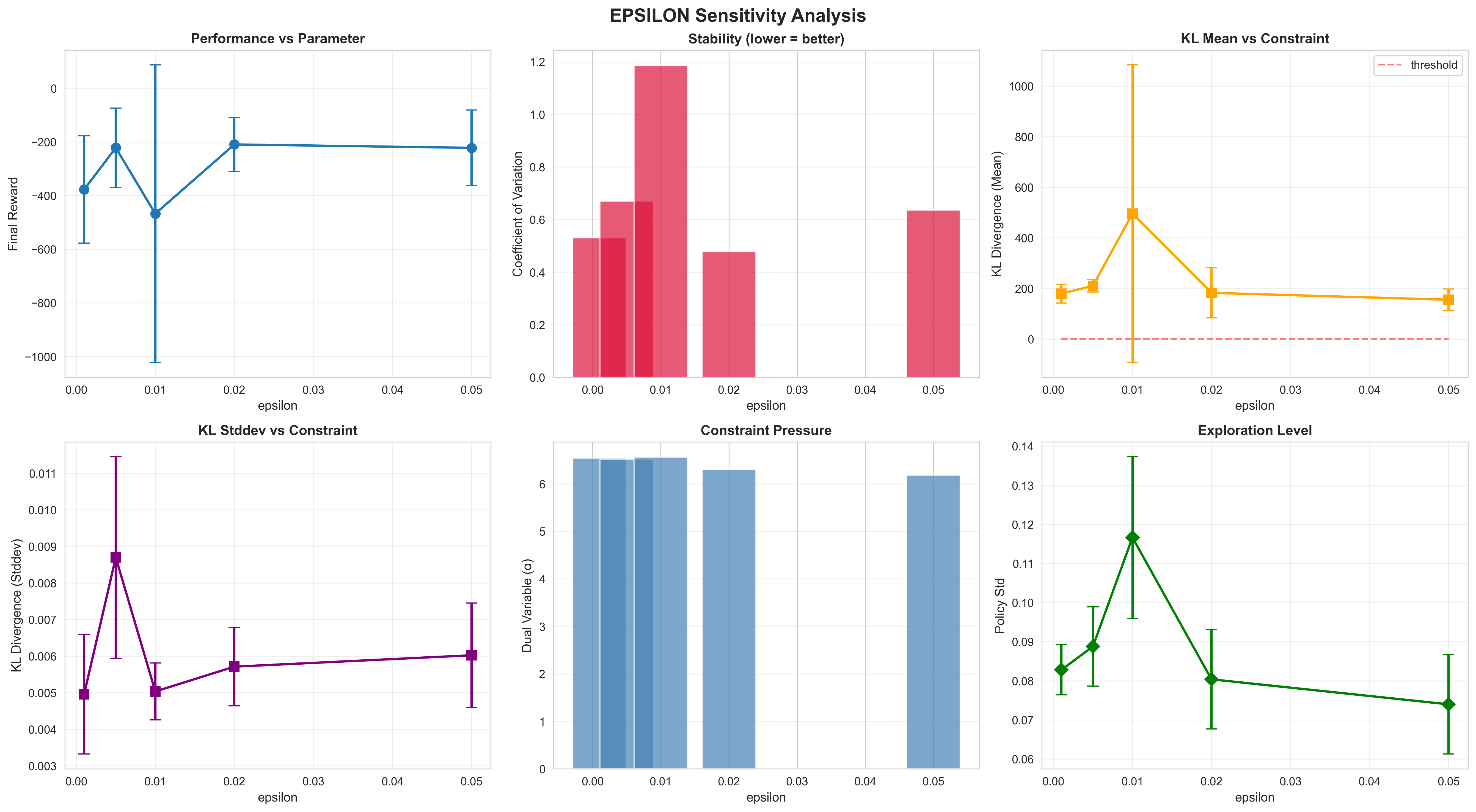 Figure 1: Six-panel analysis of epsilon sensitivity. Top row: performance vs epsilon, stability (coefficient of variation), KL mean vs constraint. Bottom row: KL stddev, dual variables (constraint pressure), policy exploration level.
| Epsilon | Success Rate | Avg Reward | Range |
|---|---|---|---|
| 0.001 | 40% | -377 | [-622, -130] |
| 0.005 | 80% | -222 | [-518, -127] |
| 0.01 | 60% | -468 | [-1570, -139] |
| 0.02 | 80% | -210 | [-404, -127] |
| 0.05 | 80% | -222 | [-503, -133] |
Surprisingly, the tightest constraint ($\epsilon$=0.001) performed worst, with only 40% of runs converging. Instead, moderate values ($\epsilon$=0.02-0.05) all achieved ~80% success rates. This contradicts the intuition that “tighter constraint = more stable learning.”
The paper’s default $\epsilon$=0.01 falls in an unstable regime here. Note: These results use slightly simplified settings:
- Buffer: 100K transitions (paper uses 2M)
- Update frequency: every step (paper uses every 100 steps)
- Network: [256, 256] actor, [512, 512] critic (paper uses [256, 256, 128] and [512, 512, 256])
The epsilon sensitivity might differ with the paper’s full configuration, though the qualitative finding—that a sweet spot exists and tighter isn’t always better—likely persists.
The KL “Violation”
The WPO paper, like many modern policy optimization algorithms, includes a KL divergence constraint (bounded by $\epsilon$) as a stability measure. While theoretically, this $\epsilon$ should enforce a hard bound on how much the policy shifts, that isn’t quite what I saw in practice.
All runs in my experiment violate the $\epsilon$ constraint by orders of magnitude—yet most still succeed. If I am not doing something wrong, this would suggest that in practice, $\epsilon$ acts less as a strict maximum bound and more as a hyperparameter that modulates the sensitivity of the dual penalty $\alpha$, which in turn controls the step size.
 Figure 2: KL divergence evolution during training for different epsilon values. Solid lines show mean across seeds, shaded regions show ±1 std. Dashed horizontal lines indicate the epsilon thresholds. All runs massively violate constraints, yet most converge.
The KL divergence starts near zero but grows to 100-300 by the end of training. For $\epsilon$=0.001, this represents a violation by a factor of 100,000. The dual variables (Lagrange multipliers α) try to enforce constraints by growing from ~1.7 to ~10.7, but cannot contain the drift. Yet 68% of runs still converge successfully. Hence, the guess about epsilon being a sensitivity parameter.
More to do
I’d like to validate the numerical correctness of my WPO update vs. the JAX implementation. This should be straightforward—run updates through both implementations with identical inputs and verify outputs. I’d be surprised if everything were numerically perfect. I also don’t know what hardware the DeepMind authors used (I’m using an oldie Intel Mac chip), but surely there are lots of things that might stray. I’m also testing with the paper’s full configuration (2M buffer, update every 100 steps, 3-layer networks) to see if epsilon sensitivity changes under those conditions.